The May 2021 numbers for the level I exams have recently been made public, a result that saw only a quarter of test takers get a pass. This is an extremely low pass rate and to put this number into context, this is the lowest pass rate in the exam’s 58-year history. By looking at the historical pass rates published by CFAI, we can see that the percentage of candidates passing the exam is between 40-50%.
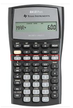
Although the CFA exam isn’t a number crunching exam, you will come across numerous questions that require the use of a calculator. Your two weapons of choice are the Texas Instrument BA II Plus and the Hewlett Packard 12C. Before buying your calculator, make sure to read the CFA Exam Calculator Policy that can be found here.
Also, if you are undecided between the two makes and you
would like to try them, both brands have apps that you can go to your phone’s App
Store and download. In terms of functionality the apps are identical to the
physical calculators.
The main purpose of this article is to make you aware of the
type of operations that you should know how to do via your calculator prior to
attempting to sit the exam.
I will be using the BA II Plus for my explanations and
examples (I will make a separate tutorial for Hewlett Packard lovers)
(1) Present Value/Future Value [Priority = High]
What is it? Other than being able to quickly perform basic
arithmetic operations on your calculator, I think this is probably one of the
most important things you will need to be able to do. You will be given the
amount of money in the bank account (PV), the prevailing interest rate and the
period of time over which the interest will compound and from this you will
need to compute the future value. You can be given any of the inputs and solve
for the missing one.
If you have started with the basics and the concept of Time Value of Money is obscure to you, you might find this article helpful.
This is also applicable to fixed income where you have the
market price of the bond, coupon payments and coupon payments frequency and you
will need to compute the IRR of the bond. You can easily compute the present
value of annuities or lease payments in Financial Reporting. Yes, simple Time
Value of Money calculations are ubiquitous on the CFA exams so let’s get started.
Examples:
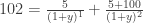
Q. A bond is trading at $102, it pays 5% coupon per annum
and matures in 2 years. What is the bond’s yield?
A. Mathematically this is what you would see if you applied the formula for calculating the yield:
If we look at the above formula for calculating the present value of a bond we can see that we are given everything except the y (for those who have studied corporate finance you can see that this is comparable to getting the IRR of a project), for the face value we can assume that it pays $100 at maturity. This gives us the below formula:
We will be using the grey buttons of our BA II Plus in the
red box.
After ensuring that you have cleared the memory (2ND function + CE|C)
Please key in the following:
2 N button
(you will see N = 2)
-102 PV (you
will see PV = -102, make sure to put the negative sign here)
5 PMT (you
will see PMT = 5, this was calculated as coupon rate * par or 5% * 100 = 5)
100 FV (you
will see FV = 100)
Now that you
have keyed in all the data, press the “CPT” key on the top left corner and
press “I/Y”. If you keyed in everything correctly you will see that your yield
is around 3.94%. If you press CPT and any of the inputs that you keyed in, you
can verify what data has been entered. For example CPT PMT will still show you
5.
This was a very brief example but try playing around with
the numbers, try changing the assumptions; for example you could easily verify
that the price of the bond falls as you increase the Yield (I/Y) by gradually
increasing the yield.
My example assumed that the coupon payment was 5% annual but
if you were told instead that the coupon was 2.5% semi-annual, remember to also
multiple the N * 2. At first, if you are not sure draw a diagram of all the
future cash flows.
(2) NPV/IRR [Priority = Medium]
What is it? Although there is an overlap with the
previous topic, I thought this part deserved its own section. With regards to overlap
I mean that we are still asking the calculator to compute present values, summing
them or solving for IRRs. For some examples you can use the PMT button as shown
above to get an answer to NPV and IRR questions. However, the limitation is
that PMT only takes the same cash flows, i.e. if you are looking for the
present value of something that pays $100 over 10 years at a fixed rate, let’s
say 5% cost of capital, then you can just key in 10 N with 5 I/Y followed by 100
PMT and 0 FV then pressing CPT PV to get your answer of -$772.17. What about a question to calculate the present
value of a project that requires an investment of -$1000 at initiation or year 0,
then pays $500 in year 1, $300 in year 2 and $400 in year 3. Your cost of
capital is 3%. This is where you cannot
use PMT and you need to key in the cash flows for discounting.
Examples: I will
use the example that I just introduced. Again this is a simplified example to
illustrate the steps and you should definitely expect harder questions.
The below formula will yield the NPV for this project:
Plugging in the numbers we get:
Now let’s obtain this number on the calculator.
Please key in the following:
CF (this button just next to the yellow 2nd key),
you should see CF(0) = 0, now just to be sure that we don’t have any data from
previous exercises, please clear the memory by pressing 2ND function
+ CE|C. Once you have done this you can press the up and down arrow keys that
are found on the top right next to the ON/OFF button to see what data is stored.
You should see CF(0) = 0, C01 = 0, F01 =0. We are ready to start:
CF(0) =
-1000 ENTER, you will see CF(0) = -1000. Press the down arrow to key in the
next cash flow.
C01 = 500 ENTER
you will see C01 = 500. If you press the down arrow key you will see F01 = 1. This
indicates the frequency of the cash flows. For example if you want the same
cash flow of 500 being paid 3 times from years 1 to 3 then you can enter 3. In
our case we have only one payment so we will keep the default value of 1 and
press the down arrow again.
Now you will
see C02 and you will be able to enter the second cash flow of 300. Repeat this for
the final cash flow of 400 and once you have entered all the cash flow data we
can compute the NPV.
You should see
C03 = 400 on your calculator. Now press the NPV button and you will see I = 0
on your calculator. Key in 5 and then press ENTER (important to note that 5
will be 5% so do not enter 0.05 otherwise you will enter 0.05%) now press the
down arrow and you will see NPV = 0. Press the CPT key on the top left and you
will see the NPV result of 93.83 and we are done. If you want to amend your
rate you can press the up arrow which will display the “I”, enter a new rate
and again press the down arrow and press CPT to calculate the NPV on the new
updated rate.
(3) Storing Results [Priority = High]
What is it? You can use the STO and RCL keys to store
calculation results and quickly recall them for future use. Before I was aware
of this feature I used to write down any interim calculation results on paper,
then I used to key in those results in my calculator to perform calculations. This
had some drawbacks as it was time consuming and prone to careless errors, not
to mention the loss of accuracy due to rounding.
Example: for
example let’s say 105.723 is your answer and you want to store this value for
future use, press STO and then any number on your number key that you want to
use to store this value. Let’s say I want the number “7” to store this value
press the key order STO 7. Now try entering any number or clearing your work
with CE|C. Now you can recall the previous number that we stored in memory by
pressing RCL and “7”, magically 105.723 will appear on your calculator.
The Time Value of Money is a core concept in finance. If you are in the early stages of your studies in the field of finance then this is a concept that you want to ensure that you understand well. In your Finance 101 class your professor might have asked you, “Would you prefer $1.00 today or would you prefer a dollar tomorrow?”. This is when students shout out “A $1.00 today is more valuable assuming no negative rates”.
They would be absolutely correct as a dollar today could be immediately deposited in a bank account to earn interest. Just to avoid adding unnecessary complications we are assuming that any payments in the future are guaranteed so there is no element of uncertainty in the expected payment; both payments are guaranteed so the only differentiator here between a dollar today and a dollar tomorrow is the opportunity cost of losing out in interest payments. So, when you are presented with this question, remember to think of what you could be doing with the money in hand. Interest earned from a bank account was just an example but what if you have a valuable project that you could invest in today to double your cash?
The Relationship Between Future Value and Present Value
So how about $0.97 today or a $1.00 in a year, which would you prefer? Now the answer to this question isn’t as obvious. We first need to make a very important remark as $0.97 and $1.00 are not two quantities that we can compare. We need to compare apples to apples. We can do this in two ways: (1) find what $0.97 would be in terms of Future Value or (2) We can find out how much $1.00 is expressed in Present Value terms. The second method is more common, especially if we think of projects which require immediate cash outlays. I call the option of getting $0.97 today Option A and the option of getting $1.00 in a year Option B.
Assuming you get 3% interest rate for depositing your cash in a bank account, you can calculate how much you would end up with in a year’s time.
A more generic way of calculating future value is:
FV = (1+r)^n * PV
where, r is the interest rate and n is the compounding frequency, in this case 1 year so n = 1. Via the above formula you can calculate the Present Value of your $1 in a year’s time.
FV = PV/(1+r)^n
therefore, 1.00/(1+0.03)^1 = 0.97087
Now we can compare like for like, for Present Value we can summarise our findings in the below table:
Present Value
Future Value
Option A
0.97
0.9991
Option B
0.97087
1
We can see that both in Present Value Terms and Future Value Terms Option B, or getting $1.00 in a year, results in us being better off.
Time Value of Money is a very powerful concept that comes up everywhere in finance. Whether it is in the form of evaluating companies and projects or finding the fair value of a complex derivative trade, we must always take into account the Time Value of Money in our models.
The Dividend Discount Model, also known as
the Gordon Growth Model is a formula that allows us to calculate the intrinsic
value of a stock. The model assumes that the fair value of a stock is the present
value of all future dividends that the company pays to its shareholders. These
dividends are discounted to present value by using the required rate of return
for the stock.
We firstly assume a model where the
dividend amounts are fixed.
As
we obtain
This result is what we call a perpetuity (an annuity that pays fixed cash flows at constant intervals until infinity). The model assumes that all company dividends are paid out therefore there is no growth in the company’s dividends. Very rarely, companies pay out all their earnings in dividends, instead a proportion of earnings are retained internally to help grow the company in the future. By adding this assumption we introduce the company’s “sustainable growth rate”. This is the constant rate at which we assume that the company and therefore the dividends will grow in the future.
As
We obtain (a growing perpetuity):
Limitations
The model isn’t applicable to
companies that currently do not pay dividends.
Dividend amounts may fluctuate over
the course of the years, so it might not make sense to assume that they are
constant. In such cases we need to look at more complicated models like a two-stage
dividend growth model.
The model requires precise estimation
as the stock price is very sensitive to the assumptions that we place for the
growth rate (g) and the required rate of return (r).
Advantages
Well known and relatively
simple to use.
Applicable to well established
companies that have a long track record of paying out dividends.
Worked Examples
Question
1
Company A pays $80 in dividends and is
expected to pay the same dividend amount forever. Investors require a 10% rate
of return for this stock. What is the intrinsic value of the stock?
‘Answer: 80/0.10 = $800
Question
2
Company B pays $25 in dividends and is
expected to pay the same dividend amount forever. Investors require a 5% rate
of return for this stock. What is the intrinsic value of the stock?
‘Answer: 25/0.05 = $500
Question
3
Company C is expected to pay a dividend of $35
next year. The company’s sustainable growth rate is 5% this growth rate is
expected to be constant. Investors require a 7% rate of return for this stock. What
is the intrinsic value of the stock?
‘Answer: 35/(0.07-0.05) = $1750
Question
4
Company C is expected to pay a dividend of $2
next year. The company’s sustainable growth rate is 2% this growth rate is
expected to be constant. Investors require a 12% rate of return for this stock.
What is the intrinsic value of the stock?
‘Answer: 2/(0.12-0.02) = $20
Feel free to post any questions you may have. Happy Studying!
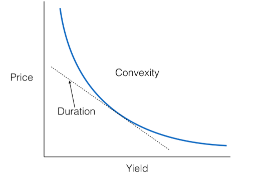
Throughout your studies of fixed income, very often you will have come across the concept of Duration. So why is it so important? Duration measures the sensitivity of your bond to changes in interest rate. Let’s say interest rates drop 1%, by using duration you can get a rough approximation of how much your bond price changes.
Bond Price and Interest Rates
Before we get started with Duration, let’s talk about bond prices and interest rates. You might have heard the expression that bond prices and interest rates are negatively related. Interest rates go down and your bond price rises, interest rates rise and your bond price drops. This is because the value of your bond is the summation of the present value of all future cash flows, so the higher your discount rate (interest rate) the lower the price of your bond.
Let’s assume that we have a bond that pays a 5% yearly coupon with a face value of 100, prevailing yields are 6% across all tenures. For simplicity, I am assuming that we have a flat yield curve with interest rates constant across all tenures.
Assumptions
Coupon
0.05
Face Value
100
Yield
0.06
Years
CFs
CFs PV
Year 1
1
5
4.7170
Year 2
2
5
4.4500
Year 3
3
5
4.1981
Year 4
4
5
3.9605
Year 5
5
105
78.4621
Bond Price
95.78764
As the the coupon rate of 5% is lower than the prevailing 6% rates, the bond is trading under par. Given the above assumptions we will calculate two key duration measures, the Macaulay Duration and the Modified Duration.
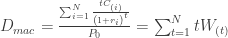
The formula for Macaulay Duration is as follows:
Where is the price of the bond, is the yield to maturity and is the year. Applying the formula in our example we get that the Macaulay Duration is 4.53 years. We can interpret this figure as the average number of years that it would take for the bond to repay the initial investment.
The formula for the Modified Duration is as follows:
Applying the formula we obtain 4.32 for the Modified Duration.
Now that we have the Modified Duration for this bond we can evaluate its sensitivity to changes in interest rates. The expected change in the bond price can be approximated by Modified Duration * Change in Rate * Bond Price. Looking at our example, if we assume that interest rates drop from 6% to 4%, then -4.32 * -0.02 * 95.79 = 8.27 is our estimated change in bond price and in reality we saw that the bond did rise by 8.66 so we can see that our approximation was quite accurate.
Duration however is only accurate for small changes in interest rates as it is only a linear approximation; we can see from the below graph that the relationship between interest rates and price is convex.
If Duration is the first order derivative between price and interest rates, we can better approximate the actual change in price by adding a second order term in the form of Convexity. I will be covering this in future posts in addition to other Duration measures such as Key Rate Duration and Effective Duration.


 is the price of the bond,
  is the yield to maturity and
  is the year. Applying the formula in our example we get that the Macaulay Duration is 4.53 years. We can interpret this figure as the average number of years that it would take for the bond to repay the initial investment.